


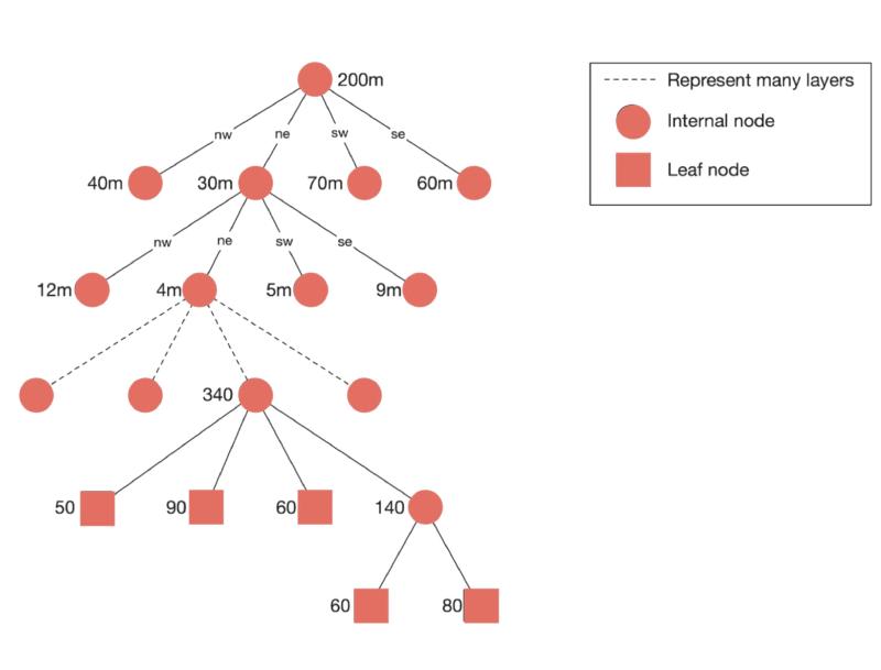
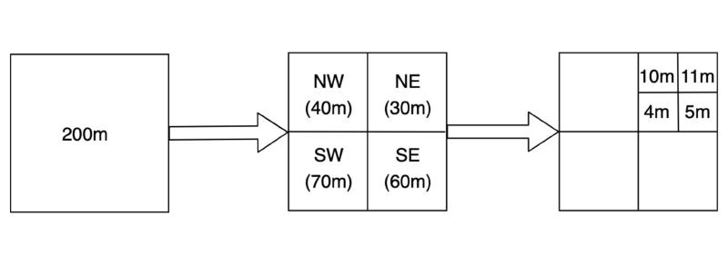
Quadtrees are a family of space-partitioning trees for 2D data. A tree starts with a single root node that represents the entire region of interest. Each subdivision splits that region into four children, usually called quadrants.
Each node is either a leaf or an internal node:
- A leaf stores information about a spatial region and has no children.
- An internal node has exactly four children and describes how the region is partitioned.
The structure is not guaranteed to be balanced. In practice, a quadtree may become very deep in dense or highly uneven data, which is why some implementations add pruning or rebuilding steps to keep it efficient.
The split does not always need to be perfectly even. Depending on the data model, regions can be divided by content rather than strict geometry. That flexibility makes quadtrees more general than a simple grid.
The closest relatives are the BSP tree in 1D/2D partitioning and the octree in 3D:
- BSP trees typically split a region into two parts.
- Octrees split 3D space into eight children.
All three structures rely on the same idea: represent space hierarchically so that searches touch fewer objects.
Use Cases #
Quadtrees are easiest to appreciate when you see where they save work. Below are a few practical examples.
Image Processing and Representation #
Starting with the entire image at the root node, the pixels can be grouped into subregions and inserted into the tree. A simple example is binary encoding: each region is represented as either 0 or 1 based on color similarity. If the source color is stored as an RGB triple with values in [0, 1], the average can be used to decide the final value and produce a grayscale approximation.
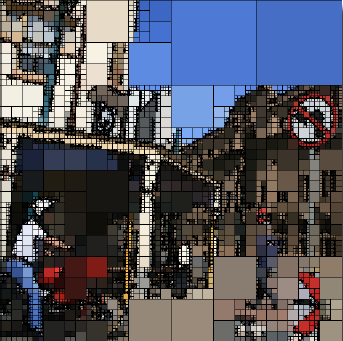
In that setting, each leaf corresponds to a region that is sufficiently uniform. This is useful for image compression because large flat areas can be stored once instead of storing every pixel individually.
The trade-off is important: if an image contains lots of gradients, texture, or noise, the tree may need to subdivide all the way down to the pixel level. In that case, the overhead of internal nodes and pointers can outweigh the benefit.
Computer Graphics #
In environments with thousands of objects, checking every object against every other one for collisions is expensive: brute force costs Θ(n²) comparisons. Quadtrees reduce that cost by storing objects in spatially localized regions.
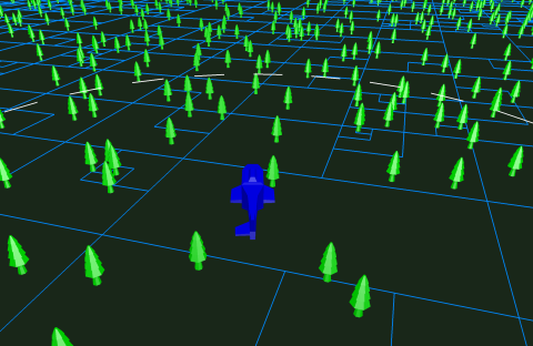
The key idea is spatial indexing: instead of comparing every object to every other object, the engine checks only the objects that share the same region or neighboring regions. The same structure can also help with visibility queries, such as identifying the portion of the world that falls inside the camera frustum.
This improves performance when the scene is fairly well distributed. If objects move rapidly or cluster tightly, however, the tree must be updated often and the benefit shrinks.
Geographic Information Systems (GIS) #
In GIS, quadtrees act like an intelligent filter. Instead of loading a massive, detailed world map all at once, the system can focus on the current region of interest, such as a city or neighborhood.
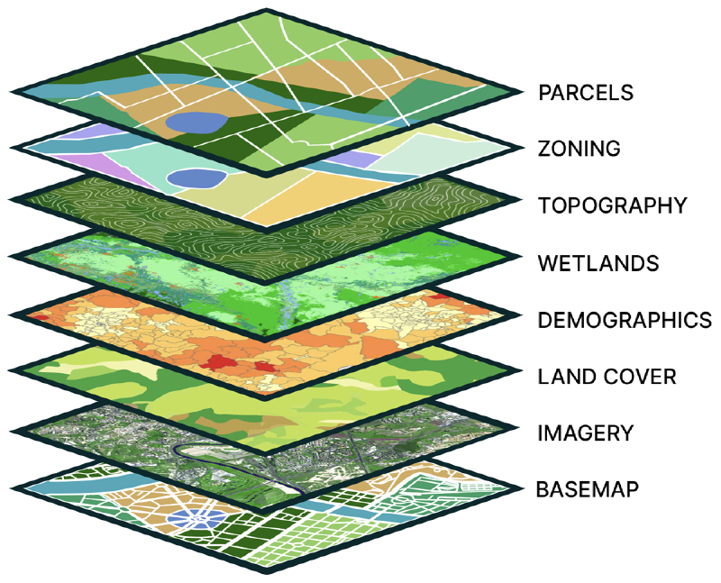
The root may represent the entire world. As the user zooms in, the map is subdivided recursively into more detailed tiles. This reduces memory pressure and avoids rendering areas the user is not currently viewing.
Quadtrees are excellent for Level of Detail (LOD) rendering, but their rigid boundaries can be a weakness when dense data lies near a division line. For complex overlapping shapes, structures such as R-trees are often a better fit.
Diffusion Models Optimization #
Traditional diffusion models often process every pixel with the same intensity, which is computationally expensive. A quadtree can help the model identify homogeneous regions such as a clear sky or a flat wall and spend less effort there. A related discussion appears in arXiv:2503.12015v1.
As shown by the Quadtree Diffusion Model (QDM) for image super-resolution, the tree can generate a spatially adaptive mask that focuses expensive computation on detail-rich regions while skipping redundant work elsewhere. The trade-off is an upfront cost to build the mask, and if the target image is uniformly complex, the tree may offer little or no savings.
Operations #
Before discussing operations, it helps to view the data as records in a spatial key space. Each node stores one record, often identified by coordinates such as x and y. A quadtree is a generalization of a binary tree with out-degree 4, where the root divides the space into four quadrants, for example NE₁, NW₂, SW₃, and SE₄.
The COMPARE(A, B) function acts as the bridge between a record and the tree. It determines which quadrant relative to record A contains record B, returning an index from 1 to 4, or 0 if the records are identical. If a quadrant is empty, it is represented as a NULL node, marking the insertion point for new data. In many implementations, this comparison is Θ(1).
In all cases, N denotes the number of nodes.
Insertion #
Insertion adds a record to the tree. The loop body is constant time, so the total cost depends on how many levels the search descends. Each iteration corresponds to one tree level.
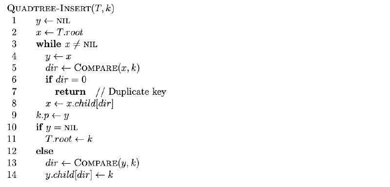
- Best case: the key is already at the root, so the operation is Θ(1).
- Average case: a reasonably balanced quadtree gives Θ(log N) depth (equivalently Θ(log_4 N) up to a constant factor).
- Worst case: a highly unbalanced tree can degrade to O(N).
Point Searching #
Point search returns the node that matches a specific coordinate pair, such as a city on a map. The recursive descent is what drives the complexity.
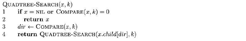
- Best case: the target is the root, so the cost is Θ(1).
- Average case: a balanced tree yields Θ(log N).
- Worst case: an extremely skewed tree requires visiting every node, which is O(N).
Regional Searching #
Regional search finds all records inside a geometric area, such as a rectangle or circle. It is useful for range queries and boolean queries over spatial attributes.
The helper tests, such as IN-REGION, FOUND, and OVERLAPS, are all constant time, so the recursion dominates.
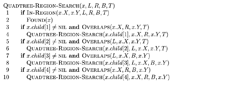
- Best case: the query region overlaps no subtree, giving Θ(1).
- Average case: this is highly query- and distribution-dependent. Finkel and Bentley observed experimentally that it inspects a small fraction of the tree. Later proofs established that for a perfectly balanced 2D point quadtree, the theoretical worst-case bound is actually O(√N + k), where k is the number of reported points.
- Worst case: if the tree is highly skewed or the query intersects almost everything, it degrades to O(N).
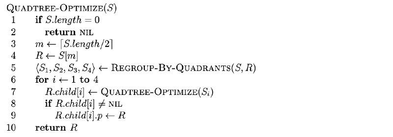
Optimization #
This operation builds a well-shaped quadtree from a static collection of records. It is ideal when the data will be queried often but does not change frequently.
The general recurrence is: T(N) = T(N₁) + T(N₂) + T(N₃) + T(N₄) + N, where N₁ + N₂ + N₃ + N₄ = N - 1.
When the data is reasonably balanced (Nᵢ ≈ N/4), this reduces to T(N) = 4T(N/4) + N, giving Θ(N log N). If one subset dominates the others at each step, the tree becomes skewed and the cost can rise to Θ(N²).
The notation S₁, S₂, S₃, S₄ is useful here because the algorithm repeatedly groups records into four quadrants, then recurses on each group.
Deletion #
Deletion removes a record from the tree, but it is difficult to do efficiently because the remaining subtrees may become disconnected. A common strategy is to take every node from the stranded subtrees and reinsert them using the standard insertion process.
Because deletion depends on reinsertion, the cost is typically:
- Best case: Θ(log N) (for example, deleting a leaf or a case with little/no reinsertion).
- Average case: O(r log N), where r is the number of reinserted nodes and the tree remains reasonably balanced.
- Worst case: O(N²)
Merging #
Merging combines two separate quadtrees into one. As with deletion, the simplest approach is usually to treat nodes from one tree as insertions into the other.
Let N be the number of nodes in the first quadtree and M be the number of nodes in the second.
- Best case: if each insertion is constant time, the total is Θ(N).
- Average case: with reasonable balance during growth, insertion costs stay logarithmic, giving O(N log(M + N)).
- Worst case: if insertion repeatedly degenerates to linear time in current tree size, the total can reach O(N(M + N)).
Comparisons #
A quadtree is conceptually similar to other spatial trees, but it trades fewer levels for more work per level. That is the central design balance: more branching, less depth.
For entity collision detection, a quadtree can reduce the number of pairwise checks dramatically. Brute force is Θ(N²), while a quadtree can approach near-linear behavior in favorable cases. In the worst case, though, it can still degrade toward O(N²).
That is why quadtrees are not always the best answer. If entities are tightly packed or move constantly, a sparse grid or another spatial index may perform better.
Conclusion #
Quadtrees are a useful data structure for representing data in two-dimensional space. Their main strength is locality: when the data is spatially clustered, the tree can cut down the search area quickly and make insertion and lookup feel almost effortless.
Their efficiency, however, depends strongly on the distribution of the data. Highly clustered datasets can produce unbalanced trees and reduce performance to O(N).
Ultimately, quadtrees remain a foundational and versatile tool across computer graphics, GIS, and image processing whenever space partitioning is the right abstraction.
Finkel, R. A., & Bentley, J. L. (1974). Quad trees a data structure for retrieval on composite keys. Acta Informatica, 4(1), 1-9.